
By Greg Marshall, Wa-chur-ed Observatory:
Greg Marshall is an amateur astro-photographer and the owner of Wa-chur-ed Observatory, a small business that offers both astro-photo art and tools for astronomy. He has an MS degree in Computer Science and 35 years of experience in electronics engineering, specializing in image processing. The actual observatory houses an AP Mach1 mount, QSI583wsg camera, and several scopes, including a 30-year-old 5.6-inch AP triplet refractor.
Throughout the years I have been active in astro-photography, my goal has been to improve the technical quality (and to a somewhat lesser extent, the artistry) of my images. The approach I have taken is to constantly analyze the defects, determine the cause of the most detrimental defect, and then work toward eliminating the problem.
A very-abbreviated list of these problems would include finding the target, focusing, various optical aberrations, guiding, focusing again, differential flexure, and so on. Eventually, this led to the ultimate challenge: seeing. Unless you are fortunate enough to live in or have access to a location with excellent typical seeing conditions, you will probably find that after all other problems have been solved, seeing still limits the sharpness of your images.
“Seeing” is the word that astronomers use to describe the steadiness of the night sky’s appearance, or to put it more simply, the amount of “twinkle” in the stars. The twinkle is caused by atmospheric turbulence and differences in the density of the air through which light must travel before we can count the photons that fall on a microscopic spot on an image sensor. It happens because light is refracted, albeit very slightly, by the air through which it passes and the amount of refraction varies with both the amount of air and its density. The density mostly varies with temperature, and as pockets of air of differing temperatures is moved through our field of view by wind, the image is distorted.
The rate at which this distortion changes can be very fast, and the magnitude of the distortion is usually great enough that it can be detected and gauged by the naked eye observer (going back to the apparent twinkling of stars). And, naturally, the effect is worse as you apply magnification.
In professional astronomy, there are two basic approaches to solving the problem of seeing: (1) space-based telescopes and (2) adaptive optics (AO). The first approach is decidedly NOT an option for the amateur astronomer, but what about the second?
“Adaptive optics” refers to a system in which the image being received through a telescope is analyzed in more-or-less real time for distortion caused by seeing, and an inverse distortion is applied to the telescope optics to remove or reduce the effect. This bit of magic is performed by something called a “wave-front corrector.”
Explaining exactly how a wave-front corrector works is beyond the scope of this article, and by that, I mean that I have no idea how it works! However, the first step in the process is quite simple: Part of the effect of changing refraction is that the position of the image can shift, so a simple tip/tilt device is driven to correct for the greatest part of the shift. This device can be either a mirror or a refractive element (i.e., a piece of glass) that moves in both X and Y axes.
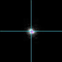
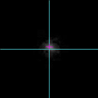
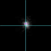
This tip/tilt part of adaptive optics, being relatively simple, has found its way into amateur equipment from a few manufacturers. Such devices have been referred to as “adaptive optics,” but that is not entirely accurate, since it does nothing to correct the distortion of a star image, but merely re-positions it so that the centroid stays in more-or-less the correct spot, thus reducing the amount of energy deposited in the wrong place. Images 1a – 1d shows a few individual frames from a video of Arcturus under
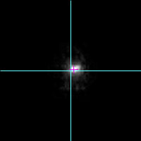
fairly poor seeing.
The blue crosshair in each frame shows where the star centroid should be and the small red crosshair shows the actual centroid. It would appear from these images that the greatest loss of image quality comes from “spreading” the energy out rather than from shifting it, but in a strictly mathematical analysis, if we want to put the greatest amount of energy into the smallest possible area (as measured by Full Width Half Maximum [FWHM] or similar metrics), being able to correct the centroid position certainly could help.
But there are lots of problems in trying to apply this theory to practice. Probably the biggest problem is speed – how quickly you can capture a guide star image, process it, and make the indicated corrections (the cycle time) compared to the speed at which
the position error changes.
To see how much benefit might be gained from a tip/tilt device, I captured sequences of video at 30 fps (frames per second) using an ordinary webcam. The lens was removed from the camera and adapter was fabricated to facilitate mounting the camera at prime focus.
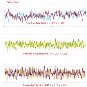
Two different techniques were used in capturing video sequences: In the first case, the AP Mach1 GTO mount was allowed to track normally so that the position errors captured would reflect the summation of all error sources. In the second case, I positioned the star on the east side of the sensor, stopped the mount’s tracking, and captured the star image as it drifted across the frame, which took about 20 seconds.
The webcam’s shutter speed (electronic shutter) was set as high as possible to get close to an “instantaneous” image of the star at each 1/30 second interval. In processing the latter sequence, the linear progression of the star in each frame was calculated from the first and last frames and this theoretically-correct position was subtracted from the measured position to arrive at the error measurement.
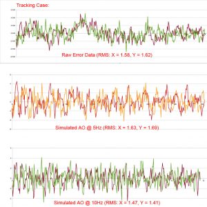
The video sequences were captured using a freeware video capture program, the individual frames were extracted using MaxIm DL, and the centroid for the star in each frame was calculated using AIP4Win. Figures 1 and 2 graph the relative error for X and Y (where X is fairly well aligned with the RA axis). For the first case (with tracking on, Figure 1) the errors are simply relative to the average position over all samples. For the second case (with no tracking, Figure 2) the “correct” position of the star is calculated by linear interpolation, as described previously, then offset by the average error, as in the tracking case.
In each figure, the top plot is the original error measurement, with X and Y axes shown in different colors. The other two plots will be described later. The first case is referred to as the “tracking” case and the other as the “drifting” case.
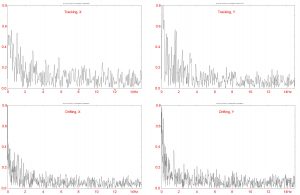
Both cases show rapid (high-frequency) changes as well as some lower-frequency components. In particular, the tracking case shows a pretty large low-frequency component in the first half of the sequence, probably due to tracking errors. I believe that the apparent correlation between X and Y during this interval is coincidental. The frequency of change in the error is important, because there is a limit on how quickly the tip/tilt system can make corrections, largely imposed by the need to expose the guide camera sensor long enough to get a good signal. To better understand the frequency of change, I ran an FFT (fast Fourier transform) on both cases, producing the plots shown in Figure 3.
As expected, the FFT plots show that some of the largest errors occur at low frequencies (less than 2 Hz), and this is especially true for the tracking case, because it includes mechanical errors in the mount. However, the mount errors should appear only in the RA axis, while the plot shows some interesting peaks in the declination axis as well (the mount was not guided, so the declination motor should not have moved). However, I did not investigate this further, because the most important conclusion to be drawn from the FFT plots is that they are probably not valid for any analysis, because there are likely to be errors at frequencies beyond half the sample rate.
When the phenomenon being studied includes frequencies above half the sample rate (in this case, probably well above the sample rate of 30 Hz) it produces aliasing that can appear as large signals at frequencies equal to the difference between the actual signal frequency and the sample rate. In other words, accurate analysis of seeing seems to require a considerably faster camera than my 30-fps webcam.
It is also interesting and instructive to note that this problem of aliasing, when the sample rate is too low, is exactly what happens when we attempt to guide a mount with a cycle time anywhere between roughly 0.01 second and 3 seconds: The “corrections” calculated by the guiding system are based on the apparent motion of seeing, but are not fast enough to actually follow the seeing and often produce error measurements that are larger than the actual error. I refer to this range of cycle times as “the dead zone”: You must either go faster and actually follow seeing accurately (as in adaptive optics), or go slower so that the effects of seeing are averaged out.
To illustrate this further and see what kind of behavior you might expect to get from an amateur-level tip/tilt AO unit, I simulated guiding on the data captured at 30 Hz. This spreadsheet simulation takes the average of N samples, where N is 30 Hz divided by the target guide rate, and applied it as a correction to the next N samples. The results of this simulation are shown in the second and third plots in Figures 1 and 2 (they are grouped together
so that you can easily compare the original errors with simulated AO residual errors).
From these plots, it is easy to see that low-frequency errors are greatly reduced, as expected, but not higher frequencies. In fact, I think you can see that large, random errors occur due to the aliasing. The RMS error value for each case is shown under the plot.
RMS is not a perfect predictor of the effect that tracking/guiding error will have on image sharpness, but it is probably the best proxy we have. For the tracking case, a simulated cycle rate of 5 Hz shows a degradation of RMS error, while a 10 Hz cycle rate shows a slight improvement. In the drifting case (removing the errors caused by the mount), the 5 Hz rate shows a small improvement in RMS error and the 10 Hz rate shows slightly more improvement.
All of the above suggests that a tip/tilt AO device operating at the kind of cycle rate you could reasonably expect to obtain with a typical amateur-level guide camera would not result in a significant improvement in image sharpness, whether by correcting for seeing or simply compensating for mount errors.
However, since the study is flawed by the limitation of my 30 Hz camera, and because simulations are often poor
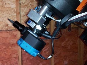
predictors of real-world behavior anyway, I decided to purchase an AO unit from Starlight Xpress (the SXV-AOQSI), knowing that the good folks at OPT Corp. would accept a return if my predictions proved correct. Image 2 shows the unit installed between my Celestron EdgeHD 8-inch with 0.7X reducer and QSI583wsg. The silver box in front of the AO unit is my PerfectStar focus motor. The guide camera is an SX Lodestar, and the mount is an AP Mach1 GTO.
This is not a review of the SX-AOQSI, so I will not go into details about the quality of the product or describe the installation process. On a positive note, I applaud Starlight Xpress for naming and describing the product honestly. They refer to it as “Active Optics” rather than “Adaptive Optics” and state clearly it can, sometimes, make some improvement with regard to seeing (the primary purpose then being to compensate for mount errors). On the negative side, I am almost always disappointed with the documentation provided with astronomy equipment,
and this product certainly did not rise above average in that regard.
The SXV-AOQSI is designed to work with QSI cameras that have a built-in guide-camera pick-off, such as mine. It is also available with a separate off-axis guider.
I have two different software solutions to control the AO unit: MaxIm DL (using a plug-in that I believe is part of the driver software from Starlight Xpress) and PHD2. I generally use PHD for conventional guiding, so I tried PHD2 first with the AO.
The PHD2 user interface for AO is easy to understand and use. It’s also very entertaining to watch the AO window as it shows dots for the current position and the desired position (the centroid of the guide star in the most recent exposure). One dot seems to be chasing the other around and never quite catches it.
I wanted to capture a real image with and without the AO to see if there was a visible difference, but found that for
most targets it is impossible to find a guide star that is bright enough to allow even a 5 Hz cycle rate. Instead, I decided to continue using Arcturus – using it as the guide star and capturing whatever star field landed on the main camera’s sensor.
I soon found that even with the extremely-short exposures possible on Arcturus (0.01 second), PHD2 could not cycle faster than around 5 to 7 Hz. The SXV-AO uses stepper motors to tip and tilt a thick piece of glass to produce shifts in the image position. There was a correction on nearly every cycle, and the device is somewhat noisy, which was disconcerting, because imaging is usually such a quiet activity. But I wondered if the noise meant that the whole imaging system wasn’t being vibrated, resulting in more degradation in image sharpness than improvement.
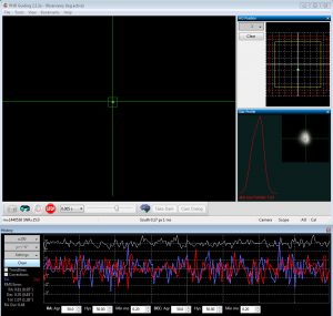
The guiding error graph was also troubling because it showed much larger errors than I would expect with normal guiding (see Figure 4).
However, this higher magnitude of errors should be expected, since we are capturing the real results of seeing, while normal guiding averages out this rapid movement.
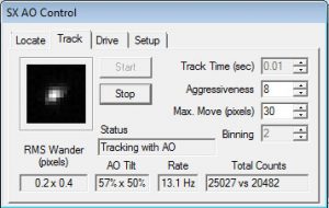
When I tried AO guiding with MaxIm DL, the results were quite different: The interface is extremely primitive and basic, but the cycle time is much better at about 12 Hz, which also seemed to reduce the mechanical noise quite a bit – perhaps because it was making smaller corrections.
Figure 5 shows the AO window under MaxIm DL while operating. Aside from being much faster than PHD2, one advantage that this software has is that it shows you the cycle rate it is achieving. For PHD2, I had to time it and could only get a rough approximation due to cycle-to-cycle variations.
You might guess from the above that PHD2’s fancy user interface limited its speed, but that does not appear to be the case. The various graph windows can be closed, but running it with no extra windows open produced very much the same cycle rate. One thing that does help a bit with the speed is using the ASCOM interface to the camera and enabling ‘use sub-frames,’ which is not available in the direct driver from Starlight Xpress. This option reduces the download time from the camera by reading only the pixels in a small area around the guide star.
Because I was using a very bright guide star, I was able to us e an exposure of 0.01 second and still get a SNR (signal to noise ratio) of about 16 with 2×2 binning. Since the typical guide star is many magnitudes less bright, a much longer exposure would be required, resulting in a reduced cycle rate.
However, it should be noted that the actual exposure time in my testing was a fairly small portion of the total cycle time. For example, at 12 Hz (using MaxIm DL) the cycle time is 1/12 or 0.083 second, so a 0.01-second exposure is just 12 percent of the cycle time. With a 0.05-second exposure, the cycle time would probably be 0.05 + (0.083 – 0.01) = 0.123, or a little more than 8 Hz (1/0.123).
However, that 5X increase in exposure time buys you only 2 magnitudes, so you should expect a much lower SNR. I have been told that AO users often guide with a SNR as low as 3. In my experience with conventional guiding, that low a SNR will produce poor results, and I would usually seek to get at least 20.
So the following results should be taken as a best-case scenario with regard to correcting for seeing. To compare image sharpness with and without the AO unit, I captured four frames using conventional guiding with a 3.5-second exposure time and four frames each with the AO controlled by PHD2 and MaxIm DL. I wanted to compare exactly the same stars, but this was not possible, because to use a 3.5-second exposure time, I had to move Arcturus completely off the guide camera sensor, so the star fields captured were very close, but not identical. The results as measured using MaxIm DL are shown below.
Cycle FWHM FWHM
Software Rate w/o AO With AO
PHD2 6 Hz 3.6 3.3 8% improvement
MaxIm DL 12 Hz 2.87 2.46 14% improvement
Note that the difference between the two software packages is not significant, as they were captured under different conditions. But the with/without AO tests were done one right after the other in each case.
Although these improvements are fairly small, they are significant when put in context. For example, I typically get no better than 2.5 arcseconds FWHM because of strong upper atmosphere winds in my area. A 10-percent improvement in this number happens only a couple of times per year, so I would pay a fairly large amount to be able to make that happen whenever I want it. On the other hand, unless I could become happy with sharp images of random star fields around very bright stars, I would not expect to actually achieve anything like a 10-percent improvement.
That is not to say that other users would also not achieve significant improvement. As I noted earlier (and as Starlight Xpress suggests), the best improvement is in compensating for mount errors, not seeing. My AP mount is much better than the mid-range mounts I have used, and I suspect that the theoretical improvement with mid-range mounts may be quite significant. Actual performance is very dependent on the choice of guide star, which involves a lot of planning and “fussing” with the camera/OAG rotation and compromise in the framing of the target.
So, my overall conclusion is that with solutions available to the amateur today it is not possible to achieve significant correction for seeing, but users of mid-range mounts might get good results with a tip/tilt AO unit. But, while the improvement is probably worth the purchase price of the AO unit, in terms of ease of use, it might be better to just move to New Mexico!
###
 The Astronomy Technology Today editorial staff would like to take this opportunity to remind you of the availability of our Solar eclipse equipment guide –The Definitive Equipment Guide to the 2017 Solar Eclipse. Our goal with the 40 page publication is to provide an easy-to-consume introduction to the technological options for viewing and imaging the Great Solar Eclipse. We cover the gamut of options available including building you own solar viewer, solar glasses, smart phones, DSLR cameras, using astronomy telescopes, solar telescopes, using binoculars, solar filters (including a DYI filter option), CCD astro cameras, astro video cameras, webcams and much more. You can view the guide on our website here – its free and there is no requirement to sign up to read the guide.